Inspiration

Imagine your worst enemy is playing a constant frequency in the center of her room. You're allowed to put speakers (which don't take up space) wherever you want in the room. The question is, what's the best place to put them and what should they play?

To be fair, this is not the question that I'll be answering in this post, but it was the inspiration. We first simplify the problem into 2D so your enemy is now vibrating a surface with constant frequency. To simulate this problem, we need to solve the wave equation, which I do in this post.

At first, I tried to figure out the finite difference equations, but I got stuck. Then, I looked it up and I found this wonderful blog post. I've rederived the equations to make sure I believed it and I wrote the code in Julia, which you can find it on GitHub. My first attempt at figuring out the finite differences is in the Python notebook, and the final code is in simulation.jl.

In action

The rederivation

See calculus notation for notation. The wave equation is $$D_{tt}u = c^2 ( D_{xx}u + D_{yy}u)$$

First, we figure out what the finite difference wave equation looks like.Since we have a second time derivative, we need to keep 2 past states to calculate the difference in the first derivative. Look at this picture ($u_{0,i,j}$ is the newest state)

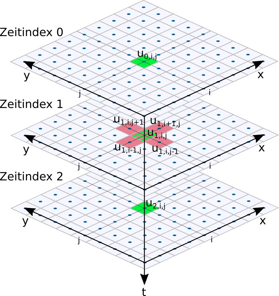
Let's do the time derivative first.$$D_tu_{1,i,j} = \frac{\Delta_t u_{1,i,j}}{dt} = \frac{u_{1,i,j} - u_{2, i, j}}{dt}$$So,$$D_{tt}u_{1,i,j} = \frac{\Delta_t D_t u_{1,i,j}}{dt}=\frac{\frac{u_{0,i,j} - u_{1, i, j}}{dt}-\frac{u_{1,i,j} - u_{2, i, j}}{dt}}{dt} = \frac{u_{0,i,j}-2u_{1,i,j}+u_{2,i,j}}{(dt)^2}$$Next, we do space derivatives (ignoring $c^2$ for now),$$ \begin{align*} D_{xx}u_{1,i,j} &+ D_{yy}u_{1,i,j} = \frac{\Delta_x D_x u_{1,i,j}}{dx} + \frac{\Delta_y D_y u_{1,i,j}}{dy}\\ &= \frac{u_{1,i-1,j} - 2u_{1,i,j} + u_{1,i+1,j}}{(dx)^2} + \frac{u_{1,i,j-1} - 2u_{1,i,j} + u_{1,i,j+1}}{(dy)^2} \end{align*}$$

Returning to the wave equation,$$ \begin{align*} D_{tt}u &= c^2 ( D_{xx}u + D_{yy}u)\\ \frac{u_{0,i,j}-2u_{1,i,j}+u_{2,i,j}}{(dt)^2} &= c^2\left(\frac{u_{1,i-1,j} - 2u_{1,i,j} + u_{1,i+1,j}}{(dx)^2} + \frac{u_{1,i,j-1} - 2u_{1,i,j} + u_{1,i,j+1}}{(dy)^2}\right)\\ u_{0,i,j} &= 2u_{1,i,j} - u_{2,i,j} +c^2 (dt)^2\left( \frac{u_{1,i-1,j} - 2u_{1,i,j} + u_{1,i+1,j}}{(dx)^2} + \frac{u_{1,i,j-1} - 2u_{1,i,j} + u_{1,i,j+1}}{(dy)^2}\right) \end{align*} $$

If we assume $dx = dy$ and $\alpha = \frac{c^2 (dt)^2}{(dx)^2}$ then$$u_{0,i,j} = 2u_{1,i,j} - u_{2,i,j} +\alpha\left( u_{1,i-1,j}+u_{1,i,j-1} - 4u_{1,i,j} + u_{1,i+1,j} + u_{1,i,j+1}\right)$$There are no $u_{0,\_,\_}$ on the RHS. Thus, every value in the newest level can be calculated by the ones in previous levels.

We deal with the boundary by only calculating u[0,1:lx,1:ly], and leaving the rest 0. So shifts are calculated like so: u[1,0:lx-2,1:ly].

Note: this is actually Verlet integration (a trick for solving for the next state in terms of the finite differences and the second derivatives).

Implementation details

We can play a frequency by resetting the value of a $u_{0,i,j}$ after the step to the value of a sine wave at the time. We can make a water droplet by setting part of the $u_{0,i,j}$ layer to a negative gaussian at a certain time step. This is achieved with put_drop!() and play_noise!() functions.